


As our year at Abertay was the last to work on the old PlayStation2 Linux Devkits, Applied Game Technologies was a last chance work on the new Vita Devkits. The purpose of this module was to choose either Augmented Reality or Stereoscopic 3D, and build a small demonstration game application to aid in discussing innovation within the chosen field.
This project was in C++, using the Abertay Framework for PlayStation Vita.
I chose to explore the idea of creating an RTS style game that would utilise Augmented Reality. The main concepts I wished to show where that of the device acting as a viewport into the game world, and interacting physically with this world to control the units.
In this demonstration application the player has to look through the PSVita to get a view of play area, and position their three towers correctly to destroy incoming enemies.

This implementation was rather difficult to use – holding a Vita in one hand while using the other hand to move the markers around. Key issues around this technologies reliance on marker identification such as limitations with tracking range, speed and stability were encountered – with possible solutions suggested.
The focus of this module was however to demonstrate how this technology could be used for further innovation. I suggested that the current movement towards headset based AR technologies coupled with gesture recognition could provide a fantastic opportunity for innovation within the RTS genre. Such upcoming technologies could allow RTS games to played within your own environment, much like a physical tabletop game – relying on user gestures for interactions rather than controllers or markers.
During the final integration process, it was necessary to finalise the details of the test environment. Structurally mostly unchanged since the conversion to Unity 5, the final details remaining represented exactly what the A.I. would be capable of ‘seeing and hearing’.
As a combination of the previously pitched ‘static’ sound emitters, I decided to place four static ‘decoys’. The player can only activate one at any time, and only when with a certain proximity – the button to activate is shown over the decoy if it can be turned on. This will represent both an audio and visual contact to the A.I. – continuously broadcasting an audio contact, and a visual contact when within the A.I.’s line-of-sight (now represented by blue arcs). The decoy stays active for a set amount of time, and is visually represented as a pair of rotating orange spotlights.

From the beginning the idea of a player launched contact had been planned. This has been implemented in the form of a green flare – launched directly from the player in the chosen direction. The range is fairly short, the player can throw over the ‘low’ (lighter grey obstacles), but not through anything higher. Representing a player-like decoy, the flare also both functions as a constant audio and visual contact – lasting a set amount of time, and only one allowed active at a time. It however is thrown, and rolls – as such is capable of movement like the player.

The final added piece of functionality was to allow the player to crouch – this will allow the player to both break LOS using low obstacles, and move silently (but slower than running). The idea being to allow some room for a player to duck behind an obstacle and break contact with the A.I. At this time I’m undecided whether I should allow the player to throw flares while concealed behind a low obstacle. It remains at this time, game play balance was never a focus for this project – just the possibilities of messing with the A.I.


After a rather significant reworking the modified ART1 network now appears to function correctly – I call it ART2 but in reality this network is far closer to its binary cousin.
Importantly the test data used represents actual vector3 positions from within my test environment – 12 floats representing 4 vector3’s – the first two allocated for visual contacts, the second two for audio contacts.
Vigilance Threshold = 0
As expected all six patterns are unique – even the first two pairs have slight differences (this was deliberate for the test data).
Vigilance Threshold = 1
The magnitude of the difference vector of the first two pairs was below 1 – these have now been accepted as members of that class and the initial node retrained (with the small differences its hard to see).

Vigilance Threshold = 28
It takes a rather high Vigilance of 28 for the final third pair to be considered a match (the x component of the second vector3’s sign was different). In practice a Vigilance this high would not be useful for my application.
The losses:
– The concept of using the dot product no longer works – vigilance is now measured by the magnitude of a difference vector between the input and the exemplar. Without the dot product this involves bypassing the normal ART architecture when a untrained or blank node is selected. In this implementation the difference vector is forced to 0’s (zero magnitude) to force a match.
– The feed-forward weight scaling equation has been altered to: value / ( 1 + the magnitude of the input vector ). This allows for negative scaling but this seems to still function correctly – same signs will result in a higher weighting, differing will lower it.
It turns out descriptions like ‘subtle changes’ or ‘more complex set-up, simpler equations’ are somewhat lacking when comparing ART1 and ART2 networks. The changes involved are significant (mostly within the F1/Input/Comparison layer), with some 15 equations including ODE’s.
I think this shows that my current ART1 network is more than likely significantly less complex than the true model – as there is only one major equation (the feed-forward weight scaling equation) along with the dot product.
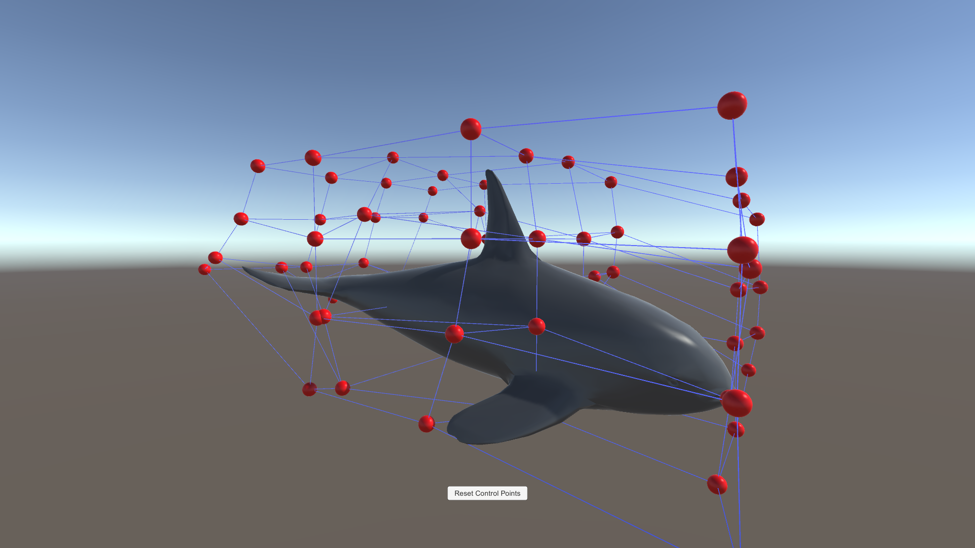
As I believed the ‘true’ ART2 architecture was far too complex, I have been pursuing modifying my existing ART1 network to accept real values. Once completed I will detail the required ‘modifications’ (hacks) required, but so far the network will accept real inputs – there is no comparison at this point (0 vigilance) – all 5 patterns are classed as new exemplars.
Even this ‘simple’ step required significant modification of the ART1 implementation – also perhaps revealing some errors within its logic.

This test data has been designed to have two sets of similar data (the first two pairs) and a final pair with some more significant differences – to test the effectiveness of the vigilance test.
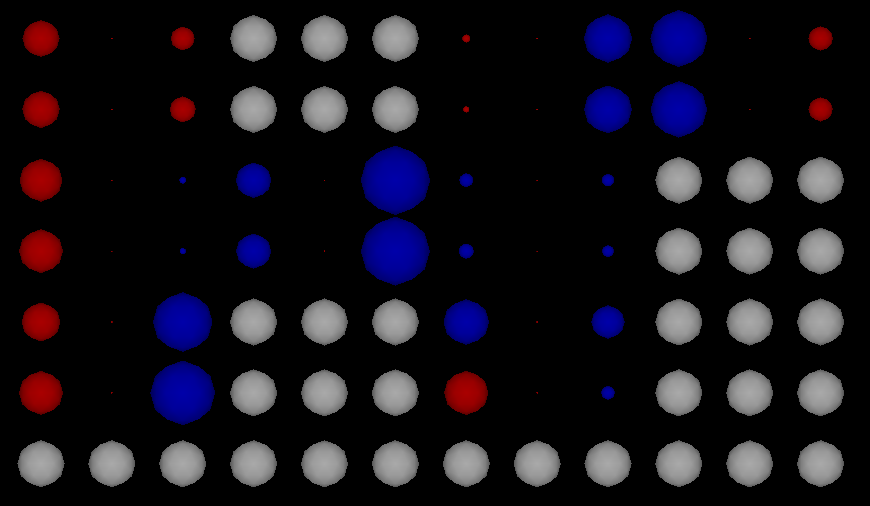
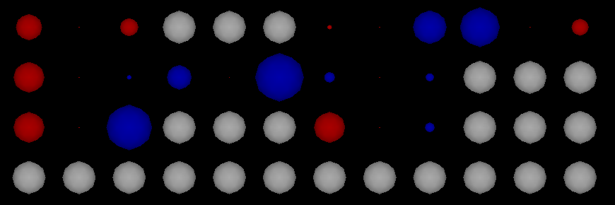
In the above image:
– white nodes represent 0’s – as the input vector has fixed length, any gaps must be filled
– blue nodes have negative values (both feedback and exemplar)
– red nodes have positive values
For non-zero nodes, the size of the sphere is the value of the feed-forward weights trained to that node – in this case they are the normalised values of the exemplar.
These screenshots show a visual representation of the output from a trained ART1 network.
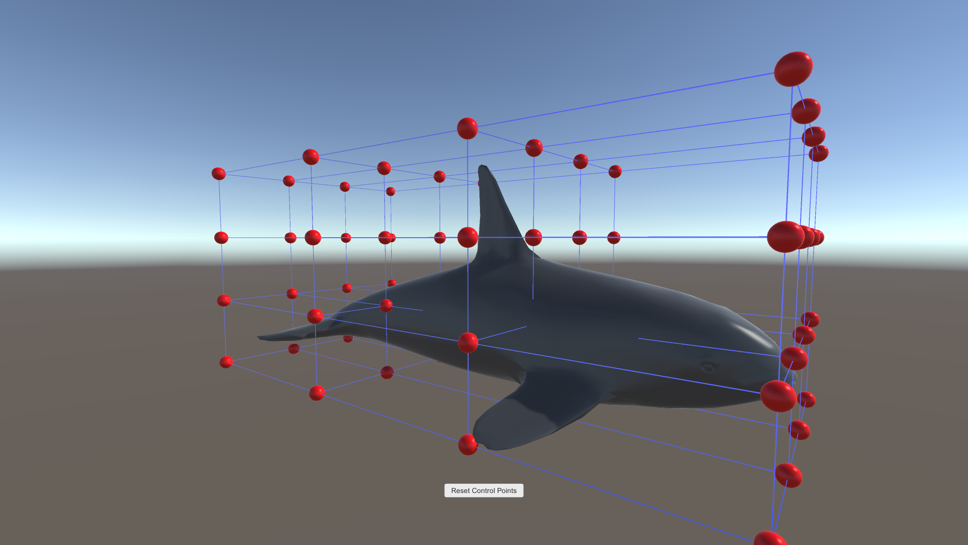
Creating a functioning ART1 network is the first step towards implementing a suitable variation within my game environment, this will likely be a modified version of an ART2 network. The key difference between ART1 & ART2 is that ART1 only accepts a binary input, where ART2 functions with real numbers.
These initial test are based around a fixed set of binary input data:
The networks outputs match those ran at vigilance thresholds of 0.3 and 0.8 – with white nodes being inactive (0), red nodes being active (1) and their size is equal to their feedforward weighting.


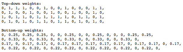 This version of the network already features some improvements over the standard model – primarily it features an extendable output node structure (recognition field). So the only two variables required for operation are the size of the test data arrays (number of binary digits – which is fixed thereafter), and the vigilance threshold value.
The recognition field is initialised with a single output node (neuron), and after this ’empty’ or ‘default’ node is trained with an exemplar pattern – a new output node is added to the field.
This limits the network by the increasing size of the recognition field and increasing time to resonate between it and the comparison field.
Currently the comparison (input) field is fixed after the network is initialised. As the size of this field is used within the feedforward weight scaling equation – it looks like this possible cannot change.
Work still progresses slowly on my ART implementation (more posts will follow), but I decided to quickly look at upgrading the project as Unity 5 released at GDC. One or two minor changes were required with the NavmeshAgent, but otherwise a simple transition.

Previously the option to render shadows had been restricted to Unity Pro licences only – no longer with Unity 5!
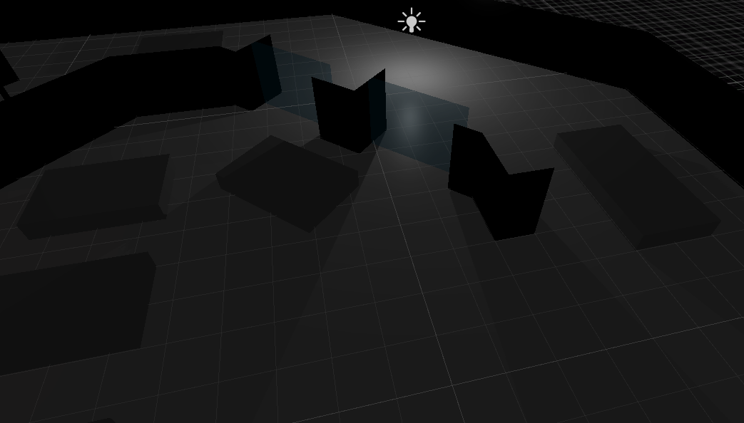
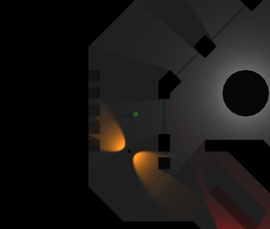
As I do not intend to further the graphics of this application, the addition of shadows and new light sources really enhances the scene. The red light here pulses like warning or alarm, while the white light flickers on and off.
The main attraction however was the blue cone light – which nicely represents the A.I.’s cone of vision, with areas in shadow correctly showing blind spots behind obstacles.
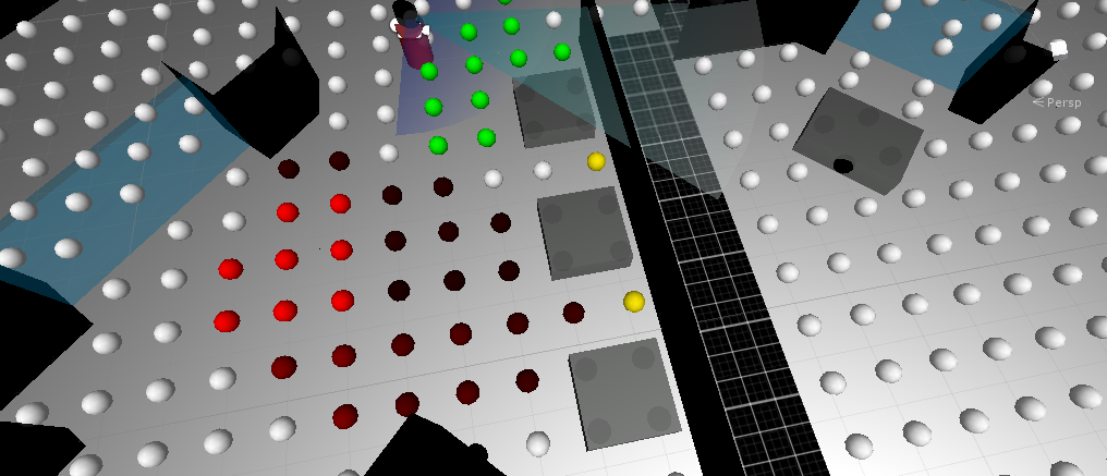
Latest implementation appears to be clustering correctly under given parameters:
– the number of ‘neighbours’ parameter appears to be one higher than expected, the images here are set at 4…
– the minimum distance between neighbours is 1.5f – this is expected as the search nodes are arranged in a 1.0f grid (save a few incorrectly placed tiles
– there does appear to be an issue with noise allocation in this implementation, a final check after the main DBSCAN loop is required to collect some missed nodes

This shot uses the same parameters but over a more complex area, again it appears to identify the search area correctly – including 3 separate clusters (each having their center shown by the blue sphere), and 10 ‘noise’ nodes.

If this currently implementation proves robust enough it will form the basis of the A.I.’s searching function:
– the DBSCAN will return two lists (clusters and noise)
– each will be given a weighted priority based on its size (always one for noise) and the distance of the A.I.’s path to its center
A new list is formed of destinations and weights – allowing the A.I. to search this area.
Larger (clusters) which are closer will have the strongest weighting.
The final thought is not simply for the A.I. to work through this list in order, but for it to choose randomly between them biased by their weighting – the largest nearest cluster would be the logical and most likely outcome, but there would be a small chance of another being chosen.
I have been working implementing a suitable search method for nearly two weeks at this point. After rewriting and improving some of the overall area detection code, the DBSCAN implementation almost looks complete.

Initially noise (yellow) nodes were being identified correctly, but clustering was definitely wrong. I have used colours here to attempt to debug the numerous clusters being generated (the actual number was often twice what the colours show).
After a fair amount of heading banging and rewriting this latest implementation appears to be giving pretty decent results, with one dodgy looking noise node to the top of the single cluster, and a rather distant looking cluster member to the bottom.

Here the algorithm has (mostly) correctly identified two main clusters, with another dodgy looking noise. Those two rogue nodes up top are still an issue.
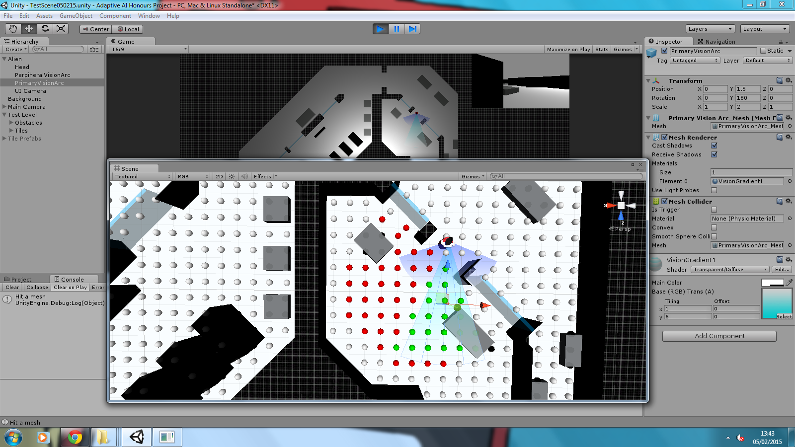
The tileset shown previously proved to have a few flaws and has been reworked slightly, but now initial functionality has been added towards implementing the required search algorithm.
Red gizmos represent those within a radius that have been highlighted to be searched, green gizmos represent those that can currently be ‘seen’ by the object. Currently this only represents the primary vision arc, and does not factor in obstacles (but that functionality has been implemented elsewhere).
Using the arc meshes for such detection proved troublesome/impossible as the project is actually in 3D rather than 2D. The work-around was:
// Get the normalised forward vector of the ‘entity’ object
Vector3 sight = forward.normalized;
// Get the normalised direction vector from the entity to this search node
Vector3 distanceVector = mSearchNodes[ i ].transform.position – center;
Vector3 direction = distanceVector.normalized;
// Dot product returns 1 (same direction), to 0 (90 degrees)
float cosine = Vector3.Dot( sight, direction );
// Use arc cos and convert from radians to degrees
float degrees = Mathf.Acos( cosine ) * Mathf.Rad2Deg;
The intended angles were about 40 degrees (primary) to 140 degrees (peripheral) achieved if the returned value was less than half of either value.
An early version of the area system has also been implemented – checking if a search area is within the radius before doing the calculation above for each search node within. Currently this relies on collider checks (returning obstacles and walls as well), but does cut down on unnecessary checks.

